

Particle Quality Control and Batch to Batch Analysis
Particle concentration measurement tells you how many particles are present in a defined volume of liquid. Expressed as particles/mL, numerical concentration connects a dispersion’s composition to practical questions about formulation, dilution, processing and batch consistency. Two samples can have similar average particle sizes yet contain very different numbers of particles.
EOS Instruments combines single particle counting with optical classification and particle size distribution analysis through SPES technologies and the Classizer™ ONE particle analyser. This approach helps laboratories investigate the whole detected sample and, where populations can be optically resolved, quantify selected components. The result is a concentration measurement that can be interpreted alongside the particles’ size and optical properties.
What numerical particle concentration measures
Numerical particle concentration, also called particle number concentration, is the number of particles per unit volume. For example a result of 1 × 10⁶ ptcs/mL means the sample contains one million particles per milliliter. To measure this number, the actual number of measured particles can be lower.
A useful concentration result therefore specifies the liquid matrix, measurement interval, dilution factor and any population selection. For mixtures, the concentration of the complete detected sample and the concentration of a selected population answer different questions.
What counts as one particle also matters. An aggregate detected as one object contributes one count, even if it contains many primary particles. A concentration change can therefore reflect aggregation, dissolution, sedimentation, particle formation or preparation losses. Interpreting the count requires knowledge of the sample and its history.
Absolute particle counting and particles per millilitre
Absolute particle counting links discrete particle events to a defined effective analysed volume, rather than reporting only relative signal intensity or a percentage distribution. The general relationship is C = N/V, where C is numerical concentration, N is the accepted particle count and V is the effective analysed volume in millilitres.
For a diluted sample, the original concentration is obtained by multiplying the measured concentration by the dilution factor. For example, 5,000 accepted particles in an effective analysed volume of 0.05 mL correspond to 100,000 ptcs/mL. A tenfold dilution gives an original sample concentration of 1,000,000 ptcs/mL, provided dilution has preserved the particle population.
These equations describe the measurement principle. They do not replace the instrument’s validated volume determination, event validation or correction procedures. Pumped volume and effective detection volume should not be assumed identical without the appropriate instrument model. Background, detection efficiency and coincidence must also be addressed in the method.
Counting statistics provide another practical limit. Under a simple independent Poisson counting model, relative counting uncertainty scales approximately as 1/√N. One hundred counts imply about 10 % relative counting uncertainty, and 10,000 counts imply about 1 %. These estimates exclude uncertainty from sampling, dilution, flow, detection and classification.
Number concentration versus mass concentration
Mass concentration describes the mass of particulate material per unit volume, commonly in mg/mL or g/L. Number concentration describes how many particles occupy that volume. Both are useful, but they are not interchangeable measures of a dispersion.
For monodisperse, compact spheres of known density, particle mass follows density multiplied by sphere volume. Because volume scales with the cube of diameter, doubling diameter increases mass per particle eightfold. At equal particulate mass and density, the smaller spheres are therefore eight times more numerous.
Converting mass into particle number becomes less reliable when size, density, composition or internal structure varies. Porous particles, hollow capsules, droplets and aggregates may require different assumptions. In a polydisperse sample, calculation should account for the distribution rather than simply applying the mean diameter. Direct number concentration avoids that particular mass-to-number conversion, while retaining the limitations of the counting method.
Reading concentration together with particle size distribution
Particle size distribution, or PSD, shows how particles are distributed across size classes. Numerical concentration adds the absolute scale. A normalised number distribution can look unchanged after dilution because the proportions remain similar, even though the particles/mL value has decreased substantially.
A single total concentration can hide changes within the size distribution. For example, the total number of detected particles can stay the same while the number of small particles falls and the number of large particles rises. Reporting concentration for each size interval makes these changes visible. Conversely, an unchanged PSD shape can accompany a loss of particles through settling or adsorption onto container walls.
Comparisons require consistent weighting and measurement limits. Number-weighted, volume-weighted and intensity-weighted distributions emphasise different aspects of the sample. A number-weighted percentage distribution alone is not an absolute concentration. For meaningful batch comparisons, retain both the absolute particles/mL result and the associated PSD, using the same analysis settings.
Measuring heterogeneous samples with SPES and the Classizer ONE
Heterogeneous dispersions may contain product particles, droplets, aggregates and unwanted particulate material together. A total concentration can obscure a change in one component if another component changes in the opposite direction. Population-specific concentration helps determine which part of the dispersion is responsible.
SPES stands for Single Particle Extinction and Scattering. In the Classizer ONE, individual particles pass through a laser measurement region in a flowing liquid. Analysis of their optical signals provides a multiparametric description that supports counting, classification and the retrieval of size and effective refractive index using appropriate models.
This combination is valuable when size alone does not distinguish the components. Particles of similar size may have different optical responses, allowing additional separation in the analysis. Optical classification does not, by itself, establish chemical identity. Assignment of a cloud to a material should be supported by sample knowledge, controls or complementary measurements.
Measurement suitability depends on particle size, optical contrast, concentration, dispersion medium and system configuration. A transparent particle and an absorbing particle need not share the same detection limit. The Classizer ONE measures particles from approximately 0.2 µm to 20 µm. The lower limit depends on the optical contrast of the particles and can be higher for weakly scattering materials, or lower for highly scattering or absorbing materials. Confirm the applicable measurement window with EOS Instruments for the intended sample.
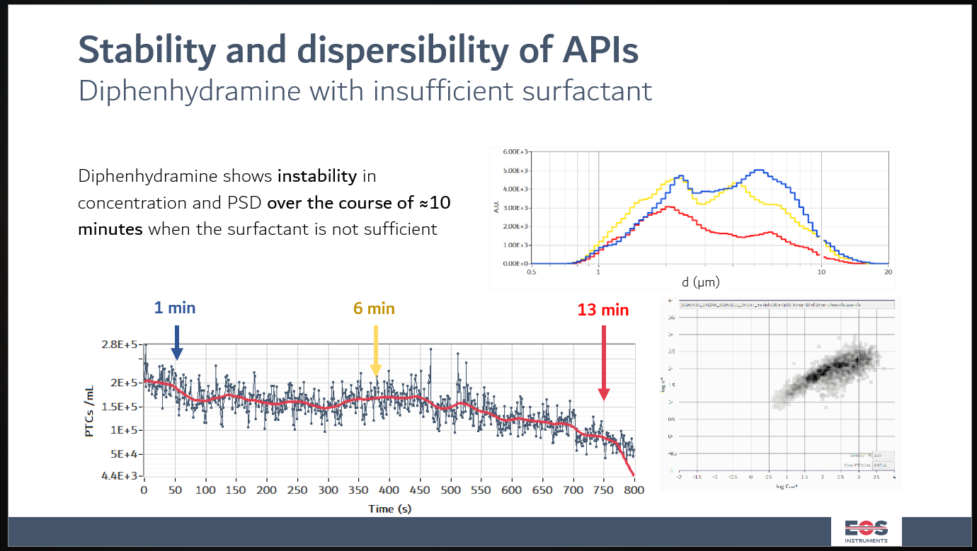
In this figure, the stability of a sample of active pharmaceutical ingredient is shown in the lower time series plot. Over time, the concentration of the sample in the measurement range decreases, and the size distribution moves to smaller particles outside the measurement range. The high sensitivity of SPES allows to track with 1 s time resolution changes in absolute concentration, in particles / mL, alongside particles’ optical properties and size distribution.
EOS Clouds and population-specific concentration
EOS Clouds represents detected particles in an optical parameter map. Distinct particle populations can form separate regions, providing a basis for selection and analysis. Classizer™ Software can retrieve numerical concentration and PSD for the whole detected sample or for a selected population.
Consider a dispersion containing polymer particles and an emulsion component. If their optical responses are sufficiently distinct, separate selections can show whether the polymer concentration changes while the droplet concentration remains stable. This is more informative than a single combined particles/mL value.
Selection boundaries should be documented and applied consistently. Overlapping clouds, weak signals or changes in optical properties can affect population assignment. A reduction in a selected population is not automatically a reduction in total particle number. Particles may have moved outside the selection. Review the complete map alongside each population result and check whether the sum of selections represents the intended sample scope.
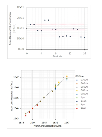
In the first graph, the concentration stability of the Classizer one along different technical and analytical replicate at different target concentrations (red lines).
In the second graph, the measured against expected concentration for a set of different polystyrene reference materials.
Comparing particle concentration measurement methods
Choose a method according to the particles, liquid matrix and decision the measurement must support. Agreement between methods requires comparable detection windows, sample preparation and definitions of particle size and counted particles.
SPES combines individual particle counting with optical classification and model-based characterisation. It is particularly relevant when the analytical question includes how concentration is distributed between optically distinguishable components. Interpretation still requires suitable detection conditions and defensible population selections.
Nanoparticle tracking analysis, NTA, follows the motion of visible individual particles to estimate hydrodynamic size and concentration. Its suitability depends on optical visibility, acquisition settings and the sample’s size and concentration range. Results should be assessed for the actual mixture rather than inferred from performance on a single reference material.
Electrical sensing zone methods count particles through changes in electrical impedance as they traverse an aperture. They provide individual particle count and volume information, with requirements related to electrolyte compatibility, aperture choice and coincidence. They offer a useful alternative when optical contrast is problematic and the sample is compatible with the measurement conditions.
Light obscuration counts and sizes particles from the reduction in transmitted light as each particle crosses a light beam. It is the compendial method for subvisible particles in injectable products, described in chapter <788> of the United States Pharmacopeia, and reports counts above defined size thresholds such as 10 µm and 25 µm. Its size scale is calibrated with polystyrene spheres. Particles with low optical contrast, such as protein aggregates, can therefore be undersized or undercounted.
Conventional dynamic light scattering (DLS) primarily evaluates fluctuations in scattered intensity to obtain hydrodynamic size information. A standard DLS size result is not a direct particle count. Specialised concentration workflows require their own assumptions and validation. Imaging methods can add morphological evidence, but concentration requires a defined sampled volume and a validated detection and segmentation process.
Applications in formulation research and quality control
In polymer dispersions and emulsions, particle concentration supports comparisons between recipes, dilution steps and production batches. Measuring particles/mL alongside PSD helps determine whether a difference reflects particle number, particle size or both. Population analysis can add context when a secondary component is present.
In milling and homogenisation studies, a change in count may accompany breakup or redistribution of particles. Interpretation should also consider sampling, agglomeration and the measurement window. Fragments below the detection limit do not contribute to the reported concentration. Count changes alone do not establish process yield or a complete particle balance.
For environmental and process liquids, concentration measurements can track changes in detected particulate load. Classification may help follow selected optical populations, while chemical identification requires appropriate supporting analysis. In research on complex biological or formulated fluids, matrix compatibility and controls are essential before attributing counts to a specific biological entity or product component.
Quality assurance for reliable concentration results
Start with representative sampling. Define mixing, sampling position, hold time and temperature where relevant. Sedimentation, creaming and adsorption can change the aliquot before it reaches the instrument. Apply a consistent preparation procedure that preserves the particles the method is intended to measure.
Assess the dilution medium and run appropriate blanks. Dilution can change ionic strength, pH or surfactant concentration and alter a dispersion. Check a dilution series where feasible. After correction, comparable original-sample concentrations should be obtained within the method’s established uncertainty. The LAD™ – Liquid Autodilutor prepares dilutions automatically and reduces manual handling in a dilution series. Investigate any deviation, and do not assume that dilution is neutral.
Control event rate and measurement duration. Excessive concentration can produce coincident events or other departures from the valid measurement regime. Insufficient counts weaken precision, particularly for rare populations. Evaluate repeatability with replicate measurements and use independent preparations when preparation variability matters.
Retain the dilution calculation, acquisition conditions, effective volume basis, analysis model, detection interval and population boundaries with the result. Establish acceptance criteria using representative samples and suitable controls.
Discuss your particle concentration measurement with EOS Instruments
Define whether the objective is total detected concentration, concentration within a size interval or concentration of a particular population. Share the dispersion medium, expected particle sizes, approximate concentration and available information about composition. EOS Instruments can assess the suitability of the Classizer ONE and discuss a measurement approach that combines particles/mL, particle size distribution (PSD) and optical classification for the analytical question.
Frequently asked questions
What does particles per millilitre mean?
It expresses particle number per unit volume of liquid. Always read the value together with its detection interval, dilution correction and population definition. A reported concentration applies to the particles detected under those conditions.
Can samples with the same particle size distribution (PSD) have different concentrations?
Yes. Normalised PSD curves describe proportions. They do not give absolute particle numbers. Two samples can have the same distribution shape while containing different numbers of particles per millilitre.
Can mass concentration be converted directly into particles per millilitre?
Only with sufficient information and justified assumptions about particle size distribution, density and structure. A single average size can give a misleading conversion for a broad distribution or a heterogeneous mixture.
Can the Classizer ONE measure individual populations in a mixture?
Classizer™ Software supports concentration analysis of selected EOS Clouds populations. Reliable separation depends on the optical distinction between components and on suitable detection and analysis conditions. Overlapping populations may require additional evidence.
Does absolute counting eliminate the need for verification?
No. Absolute concentration still requires a reliable volume basis, representative sampling and controlled detection conditions. Blanks, repeatability checks, dilution assessments and appropriate reference materials help establish whether a method is fit for its intended use.
Related posts
